Tutorials
Here we provide some tutorials on how to use M-LOOP. M-LOOP is flexible and can be customized with a variety of options and interfaces. Here we provide some basic tutorials to get you started as quickly as possible.
There are two different approaches to using M-LOOP:
You can execute M-LOOP from a command line (or shell) and configure it using a text file.
You can use M-LOOP as a python API.
If you have a standard experiment that is operated by LabVIEW, Simulink or some other method, then you should use option 1 and follow the first tutorial. If your experiment is operated using python, you should consider using option 2 as it will give you more flexibility and control, in which case, look at the second tutorial.
Standard experiment
The basic operation of M-LOOP is sketched below.
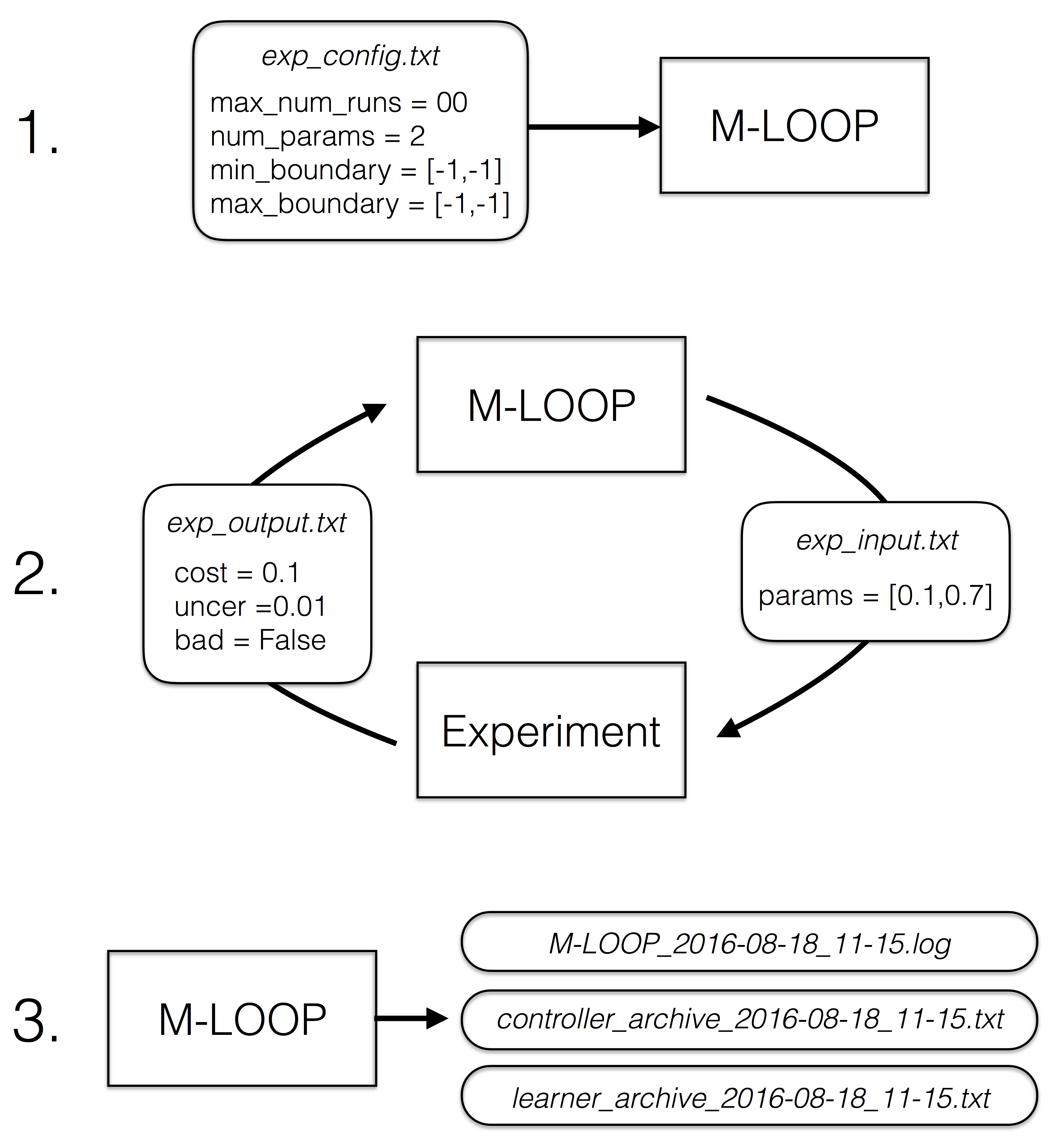
There are three stages:
M-LOOP is started with the command:
M-LOOP
M-LOOP first looks for the configuration file exp_config.txt, which contains options like the number of parameters and their limits, in the folder in which it is executed. Then it starts the optimization process.
M-LOOP controls and optimizes the experiment by exchanging files written to disk. M-LOOP produces a file called exp_input.txt which contains a variable params with the next parameters to be run by the experiment. The experiment is expected to run an experiment with these parameters and measure the resultant cost. The experiment should then write the file exp_output.txt which contains at least the variable cost which quantifies the performance of that experimental run, and optionally, the variables uncer (for uncertainty) and bad (if the run failed). This process is repeated many times until a halting condition is met.
Once the optimization process is complete, M-LOOP prints to the console the parameters and cost of the best run performed during the experiment, and a prediction of what the optimal parameters are (with the corresponding predicted cost and uncertainty). M-LOOP also produces a set of plots that allow the user to visualize the optimization process and cost landscape. During operation and at the end M-LOOP writes these files to disk:
M-LOOP_[datetime].log a log of the console output and other debugging information during the run.
controller_archive_[datetime].txt an archive of all the experimental data recorded and the results.
learner_archive_[datetime].txt an archive of the model created by the machine learner of the experiment.
If using the neural net learner, then several neural_net_archive files will be saved which store the fitted neural nets.
In what follows we will unpack this process and give details on how to configure and run M-LOOP.
Launching M-LOOP
Launching M-LOOP is performed by executing the command M-LOOP on the console. You can also provide the name of your configuration file if you do not want to use the default with the command:
M-LOOP -c [config_filename]
Configuration File
The configuration file contains a list of options and settings for the optimization run. Each option must be started on a new line and formatted as:
[keyword] = [value]
You can add comments to your file using #. Everything past the # will be ignored. Examples of relevant keywords and syntax for the values are provided in Examples and a comprehensive list of options are described in Examples. The values should be formatted with python syntax. Strings should be surrounded with single or double quotes and arrays of values can be surrounded with square brackets/parentheses with numbers separated by commas. In this tutorial we will examine the example file tutorial_config.txt
#Tutorial Config
#---------------

#Interface settings
interface_type = 'file'

#Parameter settings
num_params = 2                            #number of parameters
min_boundary = [-1, -1]                   #minimum boundary
max_boundary = [1, 1]                     #maximum boundary
first_params = [0.5, 0.5]                 #first parameters to try
trust_region = 0.4                        #maximum % move distance from best params

#Halting conditions
max_num_runs = 1000                       #maximum number of runs
max_num_runs_without_better_params = 50   #maximum number of runs without finding better parameters
target_cost = 0.01                        #optimization halts when a cost below this target is found
max_duration = 36000                      #the optimization will not start a new iteration after max_duration seconds.

#Learner options
cost_has_noise = True                     #whether the costs are corrupted by noise or not

#Timing options
no_delay = True                           #wait for learner to make generate new parameters or use training algorithms

#File format options
interface_file_type = 'txt'               #file types of *exp_input.mat* and *exp_output.mat*
controller_archive_file_type = 'mat'      #file type of the controller archive
learner_archive_file_type = 'pkl'         #file type of the learner archive

#Visualizations
visualizations = True
We will now explain the options in each of their groups. In almost all cases you will only need to adjust the parameters settings and halting conditions, but we have also described a few of the most commonly used extra options.
Parameter settings
The number of parameters and constraints on what parameters can be tried are defined with a few keywords:
num_params = 2                            #number of parameters
min_boundary = [-1, -1]                   #minimum boundary
max_boundary = [1, 1]                     #maximum boundary
first_params = [0.5, 0.5]                 #first parameters to try
trust_region = 0.4                        #maximum % move distance from best params
num_params defines the number of parameters, min_boundary defines the minimum value each of the parameters can take and max_boundary defines the maximum value each parameter can take. Here there are two value which each must be between -1 and 1.
first_params defines the first parameters the learner will try. You only need to set this if you have a safe set of parameters you want the experiment to start with. Just delete this keyword if any set of parameters in the boundaries will work.
trust_region defines the maximum change allowed in the parameters from the best parameters found so far. In the current example the region size is 2 by 2, with a trust region of 40% . Thus the maximum allowed change for the second run will be [0 +/- 0.8, 0 +/- 0.8]. Alternatively you can provide a list of values for trust_region, which should have one entry for each parameter. In that case each entry specifies the maximum change for the corresponding parameter. When specified as a list, the elements are interpreted as the absolute amplitude of the change, not the change as a fraction of the allowed range. Setting trust_region to [0.4, 0.4] would make the maximum allowed change for the second run be [0 +/- 0.4, 0 +/- 0.4]. Generally, specifying the trust_region is only needed if your experiment produces bad results when the parameters are changed significantly between runs. Simply delete this keyword if your experiment works with any set of parameters within the boundaries.
Halting conditions
The halting conditions define when the optimization will stop. We present four options here:
max_num_runs = 1000                       #maximum number of runs
max_num_runs_without_better_params = 50   #maximum number of runs without finding better parameters
target_cost = 0.01                        #optimization halts when a cost below this target is found
max_duration = 36000                      #the optimization will not start a new iteration after max_duration seconds.
max_num_runs is the maximum number of runs that the optimization algorithm is allowed to run.
max_num_runs_without_better_params is the maximum number of runs allowed before a lower cost and better parameters is found.
If a run produces a cost that is less than target_cost then the optimization will stop.
Finally, if the optimization proceeds for longer than max_duration seconds, then the optimization will end once the current iteration finishes (so the actual duration may exceed max_duration somewhat as the final iteration finishes).
When multiple halting conditions are set, the optimization process will halt when any one of them is met.
If you do not have any prior knowledge of the problem use only the keyword max_num_runs or max_duration and set it to the highest value you can wait for.
If you have some knowledge about what the minimum attainable cost is or if there is some cost threshold you need to achieve, you might want to set the target_cost.
max_num_runs_without_better_params is useful if you want to let the optimization algorithm run as long as it needs until there is a good chance the global optimum has been found.
If you have some time constraint for how long you would like the optimization to take, set max_duration.
If you do not want one of the halting conditions, simply delete it from your file. For example if you just wanted the algorithm to search as long as it can until it found a global minimum you could set:
max_num_runs_without_better_params = 50 #maximum number of runs without finding better parameters
Learner Options
There are many learner specific options (and different learner algorithms) described in Examples. Here we just present a common one:
cost_has_noise = True #whether the costs are corrupted by noise or not
If the cost you provide has noise in it, meaning the cost you calculate would fluctuate if you did multiple experiments with the same parameters, then set this flag to True. If the costs you provide have no noise then set this flag to False. M-LOOP will automatically determine if the costs have noise in them or not, so if you are unsure, just delete this keyword and it will use the default value of True.
Timing options
M-LOOP’s default optimization algorithm learns how the experiment works by fitting the parameters and costs using a gaussian process. This learning process can take some time. If M-LOOP is asked for new parameters before it has time to generate a new prediction, it will use the training algorithm to provide a new set of parameters to test. This allows for an experiment to be run while the learner is still thinking. The training algorithm by default is differential evolution. This algorithm is also used to do the first initial set of experiments which are then used to train M-LOOP. If you would prefer M-LOOP waits for the learner to come up with its best prediction before running another experiment you can change this behavior with the option:
no_delay = True #wait for learner to make generate new parameters or use training algorithms
Set no_delay to true to ensure that there are no pauses between experiments and set it to false if you want to give M-LOOP the time to come up with its most informed choice. Sometimes doing fewer more intelligent experiments will lead to an optimum quicker than many quick unintelligent experiments. You can delete the keyword if you are unsure and it will default to True.
File format options
You can set the file formats for the archives produced at the end and the files exchanged with the experiment with the options:
interface_file_type = 'txt'               #file types of *exp_input.mat* and *exp_output.mat*
controller_archive_file_type = 'mat'      #file type of the controller archive
learner_archive_file_type = 'pkl'         #file type of the learner archive
interface_file_type controls the file format for the files exchanged with the experiment. controller_archive_file_type and learner_archive_file_type control the format of the respective archives.
There are three file formats currently available: ‘mat’ is for MATLAB readable files, ‘pkl’ if for python binary archives created using the pickle package, and ‘txt’ human readable text files. For more details on these formats see Data.
Visualization
By default M-LOOP will display a set of plots that allow the user to visualize the optimization process and the cost landscape. To change this behavior use the option:
visualizations = True
Set it to false to turn the visualizations off. For more details see Visualizations.
Interface
There are many options for how to connect M-LOOP to your experiment. Here we consider the most generic method, writing and reading files to disk. For other options see Interfaces. If you design a bespoke interface for your experiment please consider Contributing to the project by sharing your method with other users.
The file interface works under the assumption that your experiment follows the following algorithm.
Wait for the file exp_input.txt to be made on the disk in the same folder in which M-LOOP is run.
Read the parameters for the next experiment from the file (named params).
Delete the file exp_input.txt.
Run the experiment with the parameters provided and calculate a cost, and optionally the uncertainty.
Write the cost to the file exp_output.txt. Go back to step 1.
It is important you delete the file exp_input.txt after reading it, since it is used to as an indicator for the next experiment to run.
When writing the file exp_output.txt there are three keywords and values you can include in your file, for example after the first run your experiment may produce the following:
cost = 0.5
uncer = 0.01
bad = false
cost refers to the cost calculated from the experimental data.
uncer, is optional, and refers to the uncertainty in the cost measurement made.
Note, M-LOOP by default assumes there is some noise corrupting costs, which is fitted and compensated for.
Hence, if there is some noise in your costs which you are unable to predict from a single measurement, do not worry, you do not have to estimate uncer, you can just leave it out.
Lastly bad can be used to indicate an experiment failed and was not able to produce a cost.
If the experiment worked set bad = false and if it failed set bad = true.
Note you do not have to include all of the keywords, you must provide at least a cost or the bad keyword set to true. For example a successful run can simply be:
cost = 0.3
and failed experiment can be as simple as:
bad = True
Once the exp_output.txt has been written to disk, M-LOOP will read it and delete it.
Parameters and cost function
Choosing the right parameterization of your experiment and cost function will be an important part of getting great results.
If you have time dependent functions in your experiment you will need to choose a parametrization of these function before interfacing them with M-LOOP. M-LOOP will take more time and experiments to find an optimum, given more parameters. But if you provide too few parameters, you may not be able to achieve your cost target.
Fortunately, the visualizations provided after the optimization will help you determine which parameters contributed the most to the optimization process. Try with whatever parameterization is convenient to start and use the data produced afterwards to guide you on how to better improve the parametrization of your experiment.
Picking the right cost function from experimental observables will also be important. M-LOOP will always find a global optimum as quickly as it can, but if you have a poorly chosen cost function, the global optimum may not be what you really wanted. Make sure you pick a cost function that will uniquely produce the result you want. Again, do not be afraid to experiment and use the data produced by the optimization runs to improve the cost function you are using.
Have a look at our paper on using M-LOOP to create a Bose-Einstein Condensate for an example of choosing a parametrization and cost function for an experiment.
Results
Once M-LOOP has completed the optimization, it will output results in several ways.
M-LOOP will print results to the console. It will give the parameters of the experimental run that produced the lowest cost. It will also provide a set of parameters which are predicted to produce the lowest average cost. If there is no noise in the costs your experiment produced, then the best parameters and predicted best parameters will be the same. If there was some noise in your costs then it is possible that there will be a difference between the two. This is because the noise might have caused a set of experimental parameters to produce a lower cost than they typically would due to a random fluke. The real optimal parameters that correspond to the minimum average cost are the predicted best parameters. In general, use the predicted best parameters (when provided) as the final result of the experiment.
M-LOOP will produce an archive for the controller and machine learner. The controller archive contains all the data gathered during the experimental run and also other configuration details set by the user. By default it will be a ‘txt’ file which is human readable. If the meaning of a keyword and its associated data in the file is unclear, just Search Page the documentation with the keyword to find a description. The learner archive contains a model of the experiment produced by the machine learner algorithm, which is currently a gaussian process by default. By default it will also be a ‘txt’ file. For more detail on these files see Data.
M-LOOP, by default, will produce a set of visualizations. These plots show the optimizations process over time and also predictions made by the learner of the cost landscape. For more details on these visualizations and their interpretation see Visualizations.
Python controlled experiment
If you have an experiment that is already under python control you can use M-LOOP as an API. Below we go over the example python script python_controlled_experiment.py. You should also read over the first tutorial to get a general idea of how M-LOOP works.
When integrating M-LOOP into your laboratory remember that it will be controlling your experiment, not vice versa. Hence, at the top level of your python script you will execute M-LOOP which will then call on your experiment when needed. Your experiment will not be making calls of M-LOOP.
An example script for a python controlled experiment is given in the examples folder called python_controlled_experiment.py, which is included below
 1#Imports for python 2 compatibility
 2from __future__ import absolute_import, division, print_function
 3__metaclass__ = type
 4
 5#Imports for M-LOOP
 6import mloop.interfaces as mli
 7import mloop.controllers as mlc
 8import mloop.visualizations as mlv
 9
10#Other imports
11import numpy as np
12import time
13
14#Declare your custom class that inherits from the Interface class
15class CustomInterface(mli.Interface):
16
17    #Initialization of the interface, including this method is optional
18    def __init__(self):
19        #You must include the super command to call the parent class, Interface, constructor
20        super(CustomInterface,self).__init__()
21
22        #Attributes of the interface can be added here
23        #If you want to precalculate any variables etc. this is the place to do it
24        #In this example we will just define the location of the minimum
25        self.minimum_params = np.array([0,0.1,-0.1])
26
27    #You must include the get_next_cost_dict method in your class
28    #this method is called whenever M-LOOP wants to run an experiment
29    def get_next_cost_dict(self,params_dict):
30
31        #Get parameters from the provided dictionary
32        params = params_dict['params']
33
34        #Here you can include the code to run your experiment given a particular set of parameters
35        #In this example we will just evaluate a sum of sinc functions
36        cost = -np.sum(np.sinc(params - self.minimum_params))
37        #There is no uncertainty in our result
38        uncer = 0
39        #The evaluation will always be a success
40        bad = False
41        #Add a small time delay to mimic a real experiment
42        time.sleep(1)
43
44        #The cost, uncertainty and bad boolean must all be returned as a dictionary
45        #You can include other variables you want to record as well if you want
46        cost_dict = {'cost':cost, 'uncer':uncer, 'bad':bad}
47        return cost_dict
48
49def main():
50    #M-LOOP can be run with three commands
51
52    #First create your interface
53    interface = CustomInterface()
54    #Next create the controller. Provide it with your interface and any options you want to set
55    controller = mlc.create_controller(interface,
56                                       max_num_runs = 1000,
57                                       target_cost = -2.99,
58                                       num_params = 3,
59                                       min_boundary = [-2,-2,-2],
60                                       max_boundary = [2,2,2])
61    #To run M-LOOP and find the optimal parameters just use the controller method optimize
62    controller.optimize()
63
64    #The results of the optimization will be saved to files and can also be accessed as attributes of the controller.
65    print('Best parameters found:')
66    print(controller.best_params)
67
68    #You can also run the default sets of visualizations for the controller with one command
69    mlv.show_all_default_visualizations(controller)
70
71
72#Ensures main is run when this code is run as a script
73if __name__ == '__main__':
74    main()
Each part of the code is explained in the following sections.
Imports
The start of the script imports the libraries that are necessary for M-LOOP to work:
#Imports for python 2 compatibility
from __future__ import absolute_import, division, print_function
__metaclass__ = type

#Imports for M-LOOP
import mloop.interfaces as mli
import mloop.controllers as mlc
import mloop.visualizations as mlv

#Other imports
import numpy as np
import time
The first group of imports are just for python 2 compatibility. M-LOOP is targeted at python3, but has been designed to be bilingual. These imports ensure backward compatibility.
The second group of imports are the most important modules M-LOOP needs to run. The interfaces and controllers modules are essential, while the visualizations module is only needed if you want to view your data afterwards.
Lastly, you can add any other imports you may need.
Custom Interface
M-LOOP takes an object oriented approach to controlling the experiment. This is different than the functional approach taken by other optimization packages, like scipy. When using M-LOOP you must make your own class that inherits from the Interface class in M-LOOP. This class must implement a method called get_next_cost_dict that takes a set of parameters, runs your experiment and then returns the appropriate cost and uncertainty.
An example of the simplest implementation of a custom interface is provided below
#Declare your custom class that inherits from the Interface class
class SimpleInterface(mli.Interface):

        #the method that runs the experiment given a set of parameters and returns a cost
        def get_next_cost_dict(self,params_dict):

                #The parameters come in a dictionary and are provided in a numpy array
                params = params_dict['params']

                #Here you can include the code to run your experiment given a particular set of parameters
                #For this example we just evaluate a simple function
                cost = np.sum(params**2)
                uncer = 0
                bad = False

                #The cost, uncertainty and bad boolean must all be returned as a dictionary
                cost_dict = {'cost':cost, 'uncer':uncer, 'bad':bad}
                return cost_dict
The code above defines a new class that inherits from the Interface class in M-LOOP. Note that this code is different from the example above; we will consider this later. It is slightly more complicated than just defining a method, however there is a lot more flexibility when taking this approach. You should put the code you use to run your experiment in the get_next_cost_dict method. This method is executed by the interface whenever M-LOOP wants a cost corresponding to a set of parameters.
When you actually run M-LOOP you will need to make an instance of your interface. To make an instance of the class above you would use:
interface = SimpleInterface()
This interface is then provided to the controller, which is discussed in the next section.
Dictionaries are used for both input and output of the method, to give the user flexibility. For example, if you had a bad run, you do not have to return a cost and uncertainty, you can just return a dictionary with bad set to True:
cost_dict = {'bad':True}
return cost_dict
By taking an object oriented approach, M-LOOP can provide a lot more flexibility when controlling your experiment. For example if you wish to start up your experiment or perform some initial numerical analysis you can add a customized constructor or __init__ method for the class. We consider this in the main example:
#Declare your custom class that inherits from the Interface class
class CustomInterface(mli.Interface):

    #Initialization of the interface, including this method is optional
    def __init__(self):
        #You must include the super command to call the parent class, Interface, constructor
        super(CustomInterface,self).__init__()

        #Attributes of the interface can be added here
        #If you want to precalculate any variables etc. this is the place to do it
        #In this example we will just define the location of the minimum
        self.minimum_params = np.array([0,0.1,-0.1])

    #You must include the get_next_cost_dict method in your class
    #this method is called whenever M-LOOP wants to run an experiment
    def get_next_cost_dict(self,params_dict):

        #Get parameters from the provided dictionary
        params = params_dict['params']

        #Here you can include the code to run your experiment given a particular set of parameters
        #In this example we will just evaluate a sum of sinc functions
        cost = -np.sum(np.sinc(params - self.minimum_params))
        #There is no uncertainty in our result
        uncer = 0
        #The evaluation will always be a success
        bad = False
        #Add a small time delay to mimic a real experiment
        time.sleep(1)

        #The cost, uncertainty and bad boolean must all be returned as a dictionary
        #You can include other variables you want to record as well if you want
        cost_dict = {'cost':cost, 'uncer':uncer, 'bad':bad}
        return cost_dict
In this code snippet we also implement a constructor with the __init__() method. Here we just define a numpy array which defines the minimum_parameter values. We can call this variable whenever we need in the get_next_cost_dict method. You can also define your own custom methods in your interface or even inherit from other classes.
Once you have implemented your own Interface running M-LOOP can be done in three lines.
Running M-LOOP
Once you have made your interface class, running M-LOOP can be as simple as three lines. In the example script M-LOOP is run in the main method:
def main():
    #M-LOOP can be run with three commands

    #First create your interface
    interface = CustomInterface()
    #Next create the controller. Provide it with your interface and any options you want to set
    controller = mlc.create_controller(interface,
                                       max_num_runs = 1000,
                                       target_cost = -2.99,
                                       num_params = 3,
                                       min_boundary = [-2,-2,-2],
                                       max_boundary = [2,2,2])
    #To run M-LOOP and find the optimal parameters just use the controller method optimize
    controller.optimize()
In the code snippet we first make an instance of our custom interface class called interface. We then create an instance of a controller. The controller will run the experiment and perform the optimization. You must provide the controller with the interface and any of the M-LOOP options you would normally provide in the configuration file. In this case we give five options, which do the following:
max_num_runs = 1000 sets the maximum number of runs to be 1000.
target_cost = -2.99 sets a cost that M-LOOP will halt at once it has been reached.
num_params = 3 sets the number of parameters to be 3.
min_boundary = [-2,-2,-2] defines the minimum values of each of the parameters.
max_boundary = [2,2,2] defines the maximum values of each of the parameters.
There are many other options you can use. Have a look at Configuration File for a detailed introduction into all the important configuration options. Remember you can include any option you would include in a configuration file as keywords for the controller. For more options you should look at all the config files in Examples, or for a comprehensive list look at the M-LOOP API.
Once you have created your interface and controller you can run M-LOOP by calling the optimize method of the controller. So in summary M-LOOP is executed in three lines:
interface = CustomInterface()
controller = mlc.create_controller(interface, [options])
controller.optimize()
Results
The results will be displayed on the console and also saved in a set of files. Have a read over Results for more details on the results displayed and saved. Also read Data for more details on data formats and how it is stored.
Within the python environment you can also access the results as attributes of the controller after it has finished optimization. The example includes a simple demonstration of this:
    #The results of the optimization will be saved to files and can also be accessed as attributes of the controller.
    print('Best parameters found:')
    print(controller.best_params)
All of the results saved in the controller archive can be directly accessed as attributes of the controller object. For a comprehensive list of the attributes of the controller generated after an optimization run see the M-LOOP API.
Visualizations
For each controller there is normally a default set of visualizations available. The visualizations for the Gaussian Process, the default optimization algorithm, are described in Visualizations. Visualizations can be called through the visualization module. The example includes a simple demonstration of this:
    #You can also run the default sets of visualizations for the controller with one command
    mlv.show_all_default_visualizations(controller)
This code snippet will display all the visualizations available for that controller. There are many other visualization methods and options available that let you control which plots are displayed and when. See the M-LOOP API for details.
