Visualizations
At the end of an optimization run a set of visualizations will be produce by default.
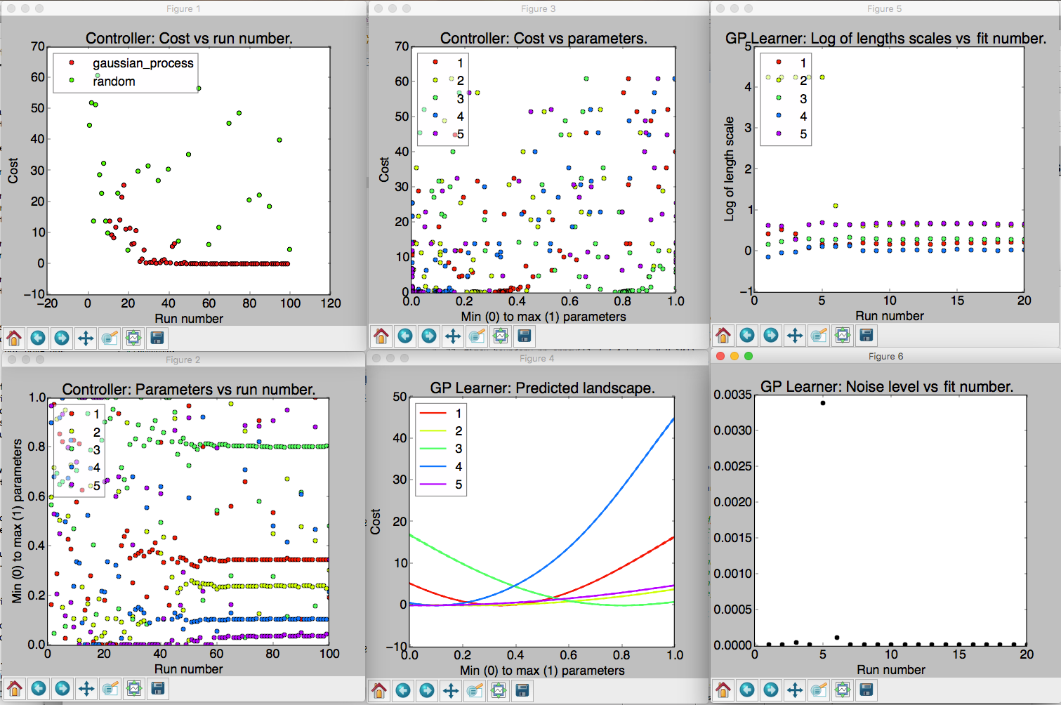
An example of the six visualizations automatically produced when M-LOOP is run with the default controller, the Gaussian process machine learner.
The number of visualizations will depend on what controller you use. By default there should be six which are described below:
- Controller: Cost vs run number. Here the returned by the experiment versus run number is plotted. The legend shows what algorithm was used to generate the parameters tested by the experiment. If you use the Gaussian process, there will also be another algorithm used throughout the optimization algorithm in order to (a) ensure parameters are generated fast enough and (b) add new prior free data to ensure the Gaussian process converges to the correct model.
- Controller: Parameters vs run number. The parameters values are all plotted against the run number. Note the parameters will all be scaled between their minimum and maximum value. the legend indicates what color corresponds to what parameter.
- Controller: Cost vs parameters. The cost versus the parameters. Here each of the parameters tested are plotted against the cost they returned as a set. Again the parameter values are all scaled between their minimum and maximum values.
- GP Learner: Predicted landscape. 1D cross sections of the landscape about the best recorded cost are plotted against each parameter. The color of the cross section corresponds to the parameter that is varied in the cross section. This predicted landscape is generated by the model fit to the experiment by the Gaussian process. Be sure to check after an optimization run that all parameters contributed. If one parameter produces a flat cross section, it is most likely it did not have any influence on the final cost. You may want to remove it on the next optimization run.
- GP Learner: Log of length scales vs fit number. The Gaussian process fits a correlation length to each of the parameters in the experiment. Here we see a plot of the correlation lengths versus fit number. The last correlation lengths (highest fit number) is the most reliable values. Correlation lengths indicate how sensitive the cost is to changes in these parameters. If the correlation length is large, the parameter has a very little influence on the cost, if the correlation length is small, the parameter will have a very large influence on the cost. The correlation lengths are not precisely estimate. They should only be trusted accurate to +/- an order of magnitude. If a parameter has an extremely large value at the end of the optimization, say 5 or more, it is unlikely to have much affect on the cost and should be removed on the next optimization run.
- GP Learner: Noise level vs fit number. This is the estimated noise in the costs as a function of fit number. The most reliable estimate of the noise level will be the last value (highest fit number). The noise level is useful for quantifying the intrinsic noise and uncertainty in your cost value. Most other optimization algorithms will not provide this estimate. The noise level estimate may be helpful when isolating what part of your system can be optimized and what part is due to random fluctuations.
The plots which start with Controller: are generated from the controller archive, while plots that start with Learner: are generated from the learner archive.
Reproducing visualizations
If you have a controller and learner archive and would like to examine the visualizations again, it is best to do so using the M-LOOP API. For example the following code will plot the visualizations again from the files controller_archive_2016-08-23_13-59.mat and learner_archive_2016-08-18_12-18.pkl:
import mloop.visualizations as mlv
import matplotlib.pyplot as plt

mlv.configure_plots()
mlv.create_controller_visualizations('controller_archive_2016-08-23_13-59.mat',file_type='mat')
mlv.create_gaussian_process_learner_visualizations('learner_archive_2016-08-18_12-18.pkl',file_type='pkl')

plt.show()
